Results
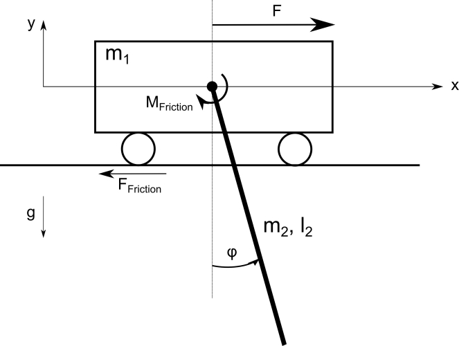
Fig. 1: Cart and pendulum experiment
Both, the collected results and evaluations as well as the Scilab/XCos libraries can be downloaded from the download area.
In this section, a few exemplary results from the cart and pendulum system are presented. The system can either be defined by its differential equations or be assembled from blocks of the XCos extension Coselica, see Fig. 2. Once the unknown system parameters have been identified, a comparison between simulation and measurement is made for verification of the identification results (Fig. 3 and Fig. 4).
[math]
\begin{bmatrix}
\tilde{m}_1+m_2 & \frac{1}{2} l_2 m_2 \cos\varphi \\
\frac{1}{2} l_2 m_2 \cos\varphi & \frac{1}{3} m_2 l_2^2
\end{bmatrix} \cdot
\begin{bmatrix}
\ddot{x} \\
\ddot{\varphi}
\end{bmatrix} =
\begin{bmatrix}
\beta u_A+\frac{1}{2} l_2 m_2 \sin\varphi \dot{\varphi}^2-\tilde{d}_1 \dot{x}\\
-\frac{1}{2} g l_2 m_2 \sin\varphi-d_2 \dot{\varphi}
\end{bmatrix}
[/math]

Fig. 2: Cart and pendulum built from Coselica blocks
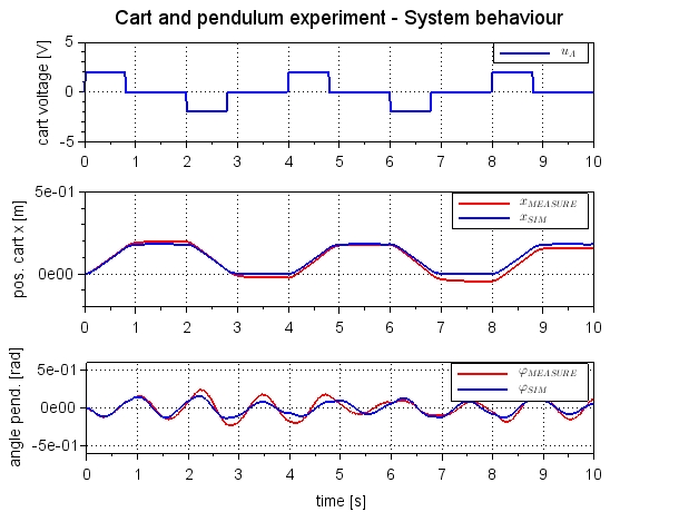
Fig. 3: Cart and pendulum – cart position and pendulum angle
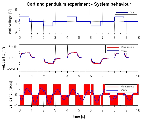
Fig. 4: Cart and pendulum – cart velocity and pendulum velocity
For calculation of a linear state controller the system has to be linearized around
[math]\textbf{q}_\textbf{s}=[x_s, \varphi_s, v_s, \omega_s]^T=[0, k\pi, 0, 0]^T, k=0,2,…[/math]
and can be written to (d2=0):
[math]
\begin{bmatrix}
\Delta \dot{x} \\
\Delta \dot{\varphi} \\
\Delta \dot{v} \\
\Delta \dot{\omega}
\end{bmatrix}
=
\begin{bmatrix}
0 & 0 & 1 & 0 \\
0 & 0 & 0 & 1 \\
0 & \frac{3 gm_2}{4 \tilde{m}_1+m_2} & -\frac{4 \tilde{d}_1}{4 \tilde{m}_1+m_2} & 0 \\
0 & -\frac{6g(\tilde{m}_1+m_2)}{l_2 (4 \tilde{m}_1+m_2)} & \frac{6 \tilde{d}_1}{l_2 (4 \tilde{m}_1+m_2)} & 0
\end{bmatrix}
\cdot
\begin{bmatrix}
\Delta x \\
\Delta \varphi \\
\Delta v \\
\Delta \omega
\end{bmatrix}
+
\begin{bmatrix}
0 \\
0 \\
\frac{4\beta}{4 \tilde{m}_1+m_2} \\
-\frac{6\beta}{l_2 (4 \tilde{m}_1+m_2)}
\end{bmatrix}
\cdot u_A
[/math]
For system identification we assume a constant but unknown pendulum length l2 which has to be estimated.
We use the the fourth system equation for identification. To get rid of the time derivatives the equation is transformed into the frequency-domain. By applying some filtering technique and inverse laplace transformation we get one algebraic equation for identification. The uknown pendulum length can be estimated using standard recursive least square algorithm.
Another possibility for parameter identification is the software tool HeuristicLab, see ModOPS Scilab/XCos library and documentation in the download area. Both methods lead to the same result, see Fig. 5 and Fig. 6.
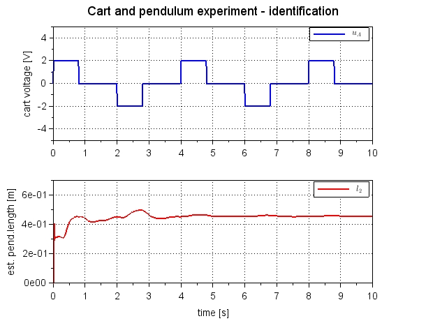
Fig. 5: Cart and pendulum – parameter identification using some filtering technique and recursive least square algorithm
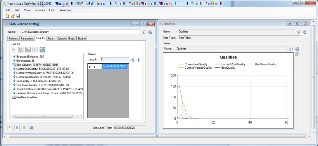
Fig. 6: Cart and pendulum – parameter identification using HeuristicLab