Design of experiments (DOE) for dynamical systems is based on the maximization of a norm of the Fisher information matrix by varying the input signal u. [math]!\underset{u}{\max}\|\textbf F(u,\textbf p)\|[/math] The Fisher information is a measure of how much information about system parameters is contained in measureable system outputs. The Fisher matrix (F) consists of the partial derivatives (sensitivity equations) of the system outputs (y) with respect to system parameters (p) and can be read as [math]!\textbf{F}(u,\textbf{p})=\sum_{k=1}^{N}\frac{\partial y}{\partial \textbf{p}}|_{\textbf{p},t_k}^{\mathrm{T}}(\sigma^2)^{-1}\frac{\partial y}{\partial \textbf{p}}|_{\textbf{p},t_k}[/math][math]!\frac{\partial y}{\partial \textbf{p}}|_{\textbf{p},t_k}=(\frac{\partial y}{\partial p_1}|_{\textbf{p},t_k},\cdots,\frac{\partial y}{\partial p_{n_P}}|_{\textbf{p}_{n_P},t_k})[/math] for a special class of systems [math]!\dot{\boldsymbol{x}}=\textbf{A}(\textbf{p})\textbf{x}+\textbf{b}u[/math][math]!y=\textbf{c}^\mathrm{T}\textbf{x}[/math] with input u and state-vector x and coefficient matrices A,b,c.

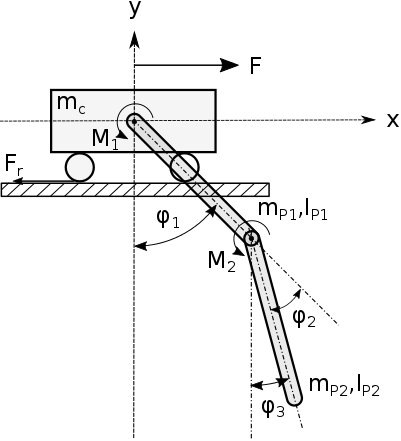
Fig. 1: Cart and double pendulum

The tool-chain for DOE aims to cover plant modeling, generation of the sensitivity equations and optimization task.

1. System modeling: System modeling is done in Scilab/Xcos by connecting physical blocks from the Modelica-based Coselica libraries. An equivalent symbolic Modelica-model is generated automatically.
2. Input design: The generated Modelica-model is imported in JModelica to generate its sensitivity differential equations automatically and perform DOE optimization to maximize the information content.

To demonstrate the DOE task using Protoframe® framework, the academic example cart with double pendulum is used.
Plant modeling is done in Scilab/Xcos using Modelica-based physical blocks, see Fig. 2.

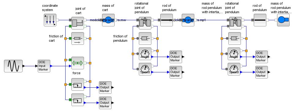
Fig. 2: Plant modeling in Scilab/Xcos

The newly created model is then loaded by the preprocessor of the Protoframe® GUI to determine system parameter values and optimization properties like final time, input- and state constraints, initial conditions, and final conditions, see Fig. 3 and Fig. 4. Additionaly, the user has to indicate which system states are measured, see Fig. 5.

Fig. 3: Protoframe GUI/preProcessor: set up model parameters

Fig. 4: Protoframe GUI/preProcessor: set up optimization parameters

Fig. 5: Protoframe GUI: set up output marker blocks

After completion of the optimization task, the optimal input signal and the corresponding information content is displayed in the GUI, see Fig. 6.

Fig. 6: Protoframe GUI: Protoframe GUI: optimal input signal and information content